00:00:10.910
Alright, I'm going to go ahead and get started. Just to let everybody know, this is my first time speaking at RubyConf and my first time speaking in general, so thank you all.
00:00:18.840
So, this is Rubik's Cube. My name is Stafford Brunk. You can find me around the internet under the handle Winged Runner 21. I work as a full-stack software engineer at Guild Education in Denver, Colorado, a startup that's striving to help working adults go back to school in an affordable manner.
00:00:31.800
However, what we don't do is anything related to Rubik's Cubes. So, why did I choose to do this project? Well, about a year ago, my wife and I were having dinner with our neighbors when their middle school-aged daughter came over. She was super excited about a Rubik's Cube-solving robot that she'd seen at a museum exhibit.
00:00:45.120
She had been learning how to solve cubes herself for the past few months and was just starting to take programming classes in school, so she was very interested in how this robot worked. I started thinking about the problem, and I thought, maybe I could figure out how to build a Rubik's Cube robot and sit down with her to explain the concepts.
00:01:01.590
I wanted to go over the differences between how a human approaches the problem of solving Rubik's Cubes and how a computer would do that. However, there was one problem: I was not an expert in these areas. In fact, I wasn't even an amateur. I'd never attempted to solve a Rubik's Cube before.
00:01:19.110
I had some robotics background and some design experience, but I hadn't done anything like this before, so I was essentially a complete novice in cubing. In the Rubik's Cube community, people who solve cubes refer to themselves as "cubers."
00:01:31.470
At this point, you all must be thinking: can I even solve a Rubik's Cube? No, I can't! But Ruby can! I'm still learning the ins and outs of solving a Rubik's Cube by hand.
00:01:38.100
This project has given me a much better idea of the fundamentals surrounding the Rubik's Cube problem set, but it has not magically bestowed upon me the ability to solve it myself.
00:01:44.910
If you'd like to follow along, all the code and associated links are posted under the Rubik's Cube repository on my GitHub account. That Google URL just takes you to the same place.
00:02:01.740
So, let's get going! Here is the general roadmap for this talk. The first thing we're going to cover is some of the basics, like terminology and movement notation. If you're a seasoned cuber, my apologies; this will be pretty basic for you.
00:02:09.120
The next step will involve looking at some strategies for solving a cube, and finally, we'll discuss what my plans are for the next steps on this project.
00:02:15.780
First up is terminology. There are essentially three basic terms that you need to be familiar with: faces, facelets, and cubelets.
00:02:21.960
First, faces refer to the individual sides of the cube. Faces are denoted relative to whichever side is closest to you, independent of color. In this instance, the yellow side of the cube is the one closest to you, so it is considered the front face.
00:02:35.640
From there, you can see the remaining faces on the cube: red is the right face, orange is the left face, blue is the upper face, green is the down face, and white is the back face. Faces are divided into nine individual facelets, which are basically the individual colored stickers on the cube.
00:02:52.410
Facelets are numbered from one to nine, starting from the upper left-hand corner and wrapping around as you go down the cube. A cubelet represents the individual colored pieces of the Rubik's Cube. There are 26 total cubelets in a 3x3 Rubik's Cube, divided into three categories: corners, edges, and centers.
00:03:05.580
You can see the corner cubelet highlighted here in pink. Corner cubelets are exactly that—the cubes located in the eight corners of the Rubik's Cube. Each corner cubelet is the intersection of three faces, giving it three possible orientations.
00:03:20.370
Let's take a look at the URF corner cubelet, as an example. If you remember from our face terminology, this represents where the yellow, red, and blue sides meet. These are the U, R, and F faces, respectively. This is the URF corner.
00:03:43.560
There are three different orientations displayed here. You can see that an individual orientation is essentially a simple rotation of the cubelet. Each corner cubelet can be oriented in a similar pattern to produce all possible orientations of the cube corners.
00:03:58.590
If you twist the one corner we have twisted here, and then another corner is twisted, that's another permutation of the cube. Note that while the corner cubelets can be placed into these orientations, you can't necessarily reach all of these orientations through legal cube moves.
00:04:05.580
This means without actually taking the cube and rotating it yourself through normal turning of the cube.
00:04:11.340
The next type of cubelet is an edge cubelet, which represents where two faces meet. Again, they're highlighted here in pink. There are 12 total edges on a 3x3 Rubik's Cube, and each edge has two possible orientations.
00:04:20.370
Here, we can see the two different orientations of the FR edge cubelet. Similar to corners, a different orientation is simply a rotation of the edge cubelet.
00:04:26.310
Just like corner permutations, the 12 edges on the cube can create all possible edge orientations.
00:04:35.520
Finally, we have center cubelets. In a 3x3 cube, there are six center cubelets. As the centers only ever touch one face, there's no orientation to worry about, as they only have one.
00:04:41.610
One of the most important things to remember about the center cubelets is that their position is essentially fixed. All corner and edge cubelets move around the centers, which serve as the axis of rotation for each individual face of the cube.
00:04:53.730
Now that we're familiar with the parts of the cube, we need to discuss how movements are denoted on the cube. For that, cubers have adopted a notation of relative movement developed by math professor David Singmaster.
00:05:05.130
I will only be talking about the basic movements here. If you're interested in more advanced cube movements, I recommend checking out Rubik's.com.
00:05:10.740
Movements are defined in terms of quarter rotations in relation to one of the cube's faces. Each movement has an optional modifier that denotes the type of movement performed.
00:05:17.460
In this example, we'll use the front or F face as the one being moved. A single letter denotes a clockwise quarter turn.
00:05:29.880
So here you can see that the F face has gone from its original solved state to having all colors rotated by 90 degrees clockwise.
00:05:36.420
There's no modifier required for this type of move. Here we can see an example of a modifier at work: F2 designates two 90-degree turns in the clockwise direction. It is possible within this notation to specify additional higher numbers, but this is rarely used as it overlaps with other notations.
00:05:46.470
For example, F4 notation would be equivalent to no movement, meaning you would do four quarter rotations and return to where you started. F prime denotes a quarter turn in the counterclockwise direction. You'll notice that this is the same as if you'd specified an F3 rotation.
00:06:01.190
Individual face movements can be chained together to create movement strings. Take a look at the movement string F R' U. We start with a solved cube on the left, execute a clockwise turn of the F face, a counterclockwise turn of the R face, and two clockwise turns of the U face. The end result is shown on the far right.
00:06:12.750
I'm pretty sure that that's the correct cube rotation, but I drew those by hand in Illustrator, so forgive me if I've got some squares out of place.
00:06:20.660
Alright, let's move on to actually solving the cube. We're going to cover three strategies here: brute force, what's commonly known as CFOP (Cross, First Two Layers, Orientation, Position), and finally, the Kociemba's two-phase algorithm.
00:06:29.340
So, why don't we just brute-force the solution to this? It's a 3x3 cube, right? It really shouldn't take us that long. Well, there are actually 43 quintillion possible permutations of a Rubik's Cube.
00:06:35.280
More precisely, 43 quintillion, 252 quadrillion, 3 trillion, 274 billion, 489 million, 856 thousand flat permutations. That is a huge number! Computing how to solve that many permutations would take you years!
00:06:53.230
This is exactly what researchers did. The upper and lower bounds on the number of moves required to solve a Rubik's Cube is known as God's number. The term comes from the idea that if God were given a scrambled Rubik's Cube, He would always solve it in the most optimal way.
00:07:01.390
The bounds were first thought to be roughly seventeen on the lower end and eighty on the high end, meaning researchers thought it would take a minimum of seventeen moves and a maximum of eighty moves when they began researching this in 1980.
00:07:19.600
It wasn't until 2010, thanks to the efforts of Thomas Rokicki, Herbert Kociemba, Morley Davidson, and John Dethridge, that the upper and lower bounds converged into a single number, which was reached via 35 CPU years of computing time donated by Google.
00:07:40.810
So, that's just how long it took them to compute that problem space, and the number is 20. All scrambled Rubik's Cubes can be solved in a maximum of 20 moves for the most optimal solution.
00:07:52.960
Researchers discovered this by computing all possible solutions to the cube and ensuring none of them required more than 20 moves. Note that they didn't have to compute all 43 quintillion different solutions to reach this conclusion due to the nature of how Rubik's Cubes move.
00:08:05.410
Some permutations are considered symmetrical to each other. For instance, if I took a Rubik's Cube and held it up and then turned it over, the solution to solving that cube would remain the same—it's just different faces on the F face.
00:08:12.560
Alright, so it took 35 CPU years to compute all the moves, which means we could just have a lookup table, right? It would just be like a giant hash and we could hit it and go—that'd be super fast.
00:08:27.910
Well, it would take a lot of space! Even if you assumed one byte per solution string—which is completely unreasonable—it would take 43,000 petabytes just to store everything!
00:08:42.210
I'm sure you've got much better things to store than Rubik's Cube movements, like your shiny new collection of air-dropped cat pictures from RubyConf.
00:08:50.520
So, the brute-force method is a no-go. Random movements would take an infeasible amount of computation time, while precomputing all possible movements would require a ton of storage—not to mention how long it would take to actually perform a lookup on such a dataset.
00:09:04.240
So, we'll have to use other strategies to solve the cube. But first, let's ask: how do humans solve a Rubik's Cube? The answer is they break it down into smaller parts.
00:09:19.200
Here's an example of a beginner strategy for solving the Rubik's Cube. It's known as the layer-by-layer strategy. This strategy is part of a set that falls under the CFOP genre. CFOP stands for Cross, First Two Layers, Orientation, and Position.
00:09:36.440
So basically, you're starting from the top of the Rubik's Cube, solving that layer, then the middle layer, then the bottom layer. This genre is popular for beginners and advanced cubing techniques.
00:09:55.760
There are some speedcubing solutions that use this method as well as some basic computer algorithms. I'm going to go through the strategy as you would solve it as a human, but I won't go into the strategy in depth.
00:10:05.520
If you'd like more information on this, again, go to Rubik's.com, where they have a great article on beginner strategies for solving the cube.
00:10:16.560
First step: make a white cross at the top. You can see that the edges and the centers are color aligned here. Next, put the corners into position, which marks the complete solving of the first layer. You can see that the orange and the green are solved while the centers remain in position.
00:10:36.740
Next is to solve the second layer. Here, I've actually flipped the cube over. This is in preparation for the next step, as the first layer would be at the bottom. The second layer is in the middle; notice how the yellow cube is in the center at the bottom.
00:10:49.490
Now we're going to solve for a yellow cross and put the edges into place. You'll notice that this closely mirrors what we did in the initial steps. Now we're going to put the corners into position, which is called orienting the corners so they are roughly where they need to be, but they are not yet solved.
00:11:05.730
Finally, we solve for the yellow corners, and we’ve got a solved cube. This seems pretty good, right? We've broken it down into smaller pieces. It's a straightforward way of doing things.
00:11:14.640
But remember that each step is a different permutation of the cube. If I were a computer solving this, I would have to compute what moves are required to go from point A to point B in the most optimal solution, and I'd have to do that for all seven steps.
00:11:31.440
To illustrate this, I have a small demo. Alright.
00:11:43.820
So this is the Rubik's Cube Web 5000. We're going to generate a random cube and it should come back really quickly. This is a very naive implementation of this algorithm. You can see that it returned with 79 moves—not too bad.
00:11:50.140
Some of these are whole cube rotations, which makes the move amount a little inflated. This is just to solve the first layer, so we'll go ahead and let that run.
00:12:00.560
You'll notice that the lights act in a slightly different order than I talked through; it's solving the white corners first and then the edges, just a slightly different ordering while performing the same algorithm.
00:12:10.480
I'm going to try this again!
00:12:15.700
Okay, that's better. Sorry about that. So, we're going to go back to computing the entire cube solution. Part of this is the library I'm using to visualize the cube, which is a project called the Rubik's Cube.
00:12:31.400
It's a pretty cool visualization, but it's a little finicky with how the solution string comes back. It'll actually change the sticker colors around, so it should be the full cube solution.
00:12:50.130
Alright, I plan to come back to this when we switch over to Kociemba's algorithm.
00:12:59.910
Alright, sorry about that! Kociemba's algorithm was created by Herbert Kociemba, a German mathematician who you may remember was part of the team that helped discover that God's number was twenty.
00:13:05.480
His algorithm is made up of two phases. The first phase solves the cube into a known state, allowing the second phase to require a considerably smaller subset of moves needed to finalize the solving.
00:13:21.350
Just as an example, the first two layers solution will solve the cube into a given state. In this instance, the first phase finds the solution to the first two layers, while the second phase solves the rest of the cube.
00:13:39.290
For our problem set, we're looking for the most optimal solution for solving the first two layers, and from there, we're seeking the most optimal solution to solve the remaining layer.
00:13:54.450
Contrast that to the layer-by-layer solution we just discussed: while theoretically sound, you can see that if God's number is 20, then phase one plus phase two should equal a maximum of 20.
00:14:07.080
Yet, even with the optimal moves we've been getting back, we were well above 20.
00:14:20.480
So, in order to solve this, we should probably use a tree—more specifically, a game tree.
00:14:36.640
What is a game tree, you might ask? For those who are new to programming, you may not be familiar with trees at all. So let’s go over a small example.
00:14:47.550
Okay, good. This is a game tree for tic-tac-toe. As you can see, the initial state of the tree is the empty board—that's the root. Each additional depth of the tree has leaves, which represent new states in the game.
00:15:02.390
Each edge or line that connects a leaf corresponds to a move in the game and each level of the tree is considered an additional depth. The idea is to search the tree until you find a winning state.
00:15:15.600
There are two general ways of performing this search: breadth-first search and depth-first search.
00:15:31.920
Breadth-first search goes across the tree first, searching at depth zero and then depth one, going from left to right.
00:15:40.330
As you can see, each leaf is checked for the finished solution. If you find that solution, you're done and don’t need to go any further.
00:15:56.230
On the other hand, depth-first search means you go all the way down the left side of the tree as far as you can, then you start coming back up, continuing to check until all leaves have been traversed.
00:16:07.960
The problem with the game tree is that usually, all possible permutations of the game are impossible or highly difficult to build into a tree.
00:16:21.950
In tic-tac-toe, you can probably do it relatively easily. However, you cannot place 43 quintillion different combinations into a tree structure in memory.
00:16:34.440
So we need to create some sort of heuristic to make our search more efficient. One way to do that is to limit the depth of the search.
00:16:47.870
Since we know God's number specifies that all cubes can be solved in a maximum of 20 moves, we can set our search depth limit to 20.
00:17:04.650
Another problem with the game tree, as we have it set up, is that you have to make a trade-off regarding how close to a solved Rubik's Cube you are.
00:17:16.210
For example, if all you did was perform one turn on the cube, you'd expect that solution to be at a depth of 1 on the tree.
00:17:30.540
However, if you do a depth-first search, it is possible you'll be waiting a long time compared to if you were doing breadth-first search.
00:17:43.860
It would be great if we could minimize that trade-off. In fact, if we did a breadth-first search, we could hit the solution move on the fifth leaf iterated here. But, if we were doing a depth-first search, we would have to go all the way down and up.
00:17:58.660
This big difference in time can be extrapolated to the Rubik's Cube problem set.
00:18:10.540
We can use a technique called iterative deepening to hybridize the differences between depth-first and breadth-first search.
00:18:22.040
Let's continue to use the first two layers as an example. Let's say it takes 15 moves to solve the first phase and 11 moves to solve the last layer, giving us a total of 26 moves.
00:18:32.760
Iterative deepening allows us to use less optimal solutions for phase one and check to see if we can generate a shorter phase two.
00:18:43.520
So, let's visualize this: in the first row, we have our optimal 15 moves for phase one and then 11 moves for the remainder of phase two, totaling 26 moves. Then we check: maybe 16 moves in phase one generates a shorter phase two; maybe 17, 18, or 19, etc., until we hit 26 total moves in phase one and zero in phase two.
00:19:06.320
Eventually, we are going to arrive at a point where we can't find a more optimal solution, perhaps because our algorithm times out or we're at a depth limit in our search.
00:19:18.750
At that point, we can take our phase one total move count as it is, and phase two will be zero. In practice, when getting close to this bound, the last few moves in phase one often equate to the first few moves found in phase two.
00:19:27.440
Alright, how does this all relate to Kociemba's algorithm? Instead of using F2L or the first two layers as its initial state for phase one, Kociemba's algorithm solves the cube into a known state called G1.
00:19:44.300
The properties of G1 mean that all corners and edges are oriented, and all middle layer edges are already in the middle layer.
00:20:04.170
In simpler terms, corners and edges are oriented so they are positioned roughly where they need to be at the solve state. Middle layer edges are already in the middle layer, which means they need to end up there but may not necessarily be on the target side.
00:20:16.830
The idea around solving to this initial state is that only a small subset of moves are required to finish solving the cube.
00:20:30.580
From state G1, you'll find that only the moves U, D2, F2, L2, and B2 are needed to transition to the solved state.
00:20:43.240
This cube is not in the G1 state, but it illustrates various edges and corners that are oriented.
00:20:56.050
Alright, let’s hope this time we perform a little better. We'll be using Kociemba's algorithm, and I’m sending it to search to a depth of 21, which is just one more than God's number.
00:21:09.470
The reasoning is that my implementation of Kociemba's algorithm currently needs some optimization, and having an extra piece of depth greatly helps the amount of time it takes to search.
00:21:27.660
Sometimes it takes a little while. Alright, we're back, and we found a 20-move solution, which took about 14 seconds to compute. Sometimes, it can be much faster.
00:21:41.710
There! A 21-move solution! The longest I’ve seen for my implementation is approximately 45 seconds.
00:22:07.200
Alright, onto the next steps for the project. I based the initial implementation on reference Python implementations by a couple of different individuals.
00:22:23.150
One was by the initial author of the algorithm, who ported his Python implementation from his Java version, and the second was from someone named Maxim SOI.
00:22:39.160
He's developed various cube-solving robots and has some novel ideas regarding robotic mechanics and efficient methods for grabbing and releasing the cube.
00:22:51.700
I ported the code fairly directly, converting idiomatic Ruby where it seemed low-risk, but in general, it retained a Pythonic structure.
00:23:01.850
My next task is to optimize the code for the Ruby interpreter.
00:23:08.470
One aspect of this algorithm that it makes prolific use of is while loops. I've included a lot of while true loops, while RuboCop recommends using loop instead.
00:23:24.900
However, for low-level tests, using loop is actually slower than while true. If you remember, loop requires a block, which creates a new variable context each time, while while just loops directly.
00:23:36.580
This implies that my algorithm may not end up being idiomatic Ruby. I plan to write a benchmarking suite to evaluate any performance penalties idiomatic Ruby might incur.
00:23:51.130
Another enhancement I’d like to implement is symmetry detection. If you recall, I mentioned this before: basically detecting if a cube state has been rotated and trying to short-circuit some of my tree searching.
00:24:07.730
The algorithm contains baseline features for this but requires further development.
00:24:20.400
There’s also a newer implementation of Kociemba’s algorithm called min2phase, which you can find in the GitHub link.
00:24:36.840
It creates the initial state of more than just G1 and includes alternative initial states and methods to prune the decision tree.
00:24:51.490
I haven't delved deeply into that yet, but it would be interesting to see what sorts of optimizations I can derive from it.
00:25:02.150
Lastly, I mentioned a robot at the beginning of this talk, and I have done significant initial work on the robot setup. The functionality can be boiled down to three steps: read the cube state, compute the solution, and finally, solve the cube.
00:25:16.840
For this instance, we use OpenCV to read the cube state and employ Kociemba's algorithm or a modified version to calculate the solution.
00:25:31.360
We then translate that move set into motor movements. You can see a screenshot here of some progress I made to read the facelets using OpenCV.
00:25:43.820
The facelets are highlighted and correctly detected; there’s still work needed around dynamically compensating for variable lighting conditions and doing some refactoring, but it’s functioning well.
00:26:00.700
The only area I have not quite nailed down is that the OpenCV bindings for Ruby do not handle live video streams particularly well.
00:26:15.120
I think I may need to switch to something more akin to C++ to better manage the data structures, as translating to Ruby objects is simply too slow for real-time video processing.
00:26:31.180
So, the next steps will be continuing with Kociemba's algorithm, finalizing the robot setup, and translating movement strings into some type of motor functions.
00:26:41.080
I have started to design the mechanics of the robot, and you can find some STL files in the GitHub repository. These are files that you 3D print, which pertain to the cube gripper and the mounting gears.
00:27:02.220
Eventually, I hope to publish a full bill of materials there and provide instructions for others to build their own robots, how to run it, etc.
00:27:20.340
I’ve also begun implementing motor functionality; however, I checked existing projects like the R2 gem, and they don’t quite implement stepper motors.
00:27:33.910
I require fine-grained motor control to ensure that I'm turning exactly 90 degrees, and thus, I am going to implement my own lightweight solution.
00:27:43.540
There's already a library available on my GitHub account called LiveMPS. This is a USB interface for the I2C bus, which allows embedded devices to communicate with each other.
00:27:57.950
It’s essentially a C library wrapped using FFI, and I've designed the constructs to be compatible with the existing I2C gem—that way.
00:28:09.660
Eventually, I hope to integrate that into the motor controller, allowing it to fit seamlessly into existing projects.
00:28:19.300
Instead of relying on something like a Raspberry Pi, you can connect a device that Adafruit provides to a USB port on your computer and get the exact same functionality.
00:28:32.000
Alright, thanks! That’s all I have.