RubyConf 2019
Algorithms: CLRS in Ruby
Algorithms: CLRS in Ruby
by Brad GrzesiakThe video presented by Brad Grzesiak at RubyConf 2019 centers on implementing algorithms from the renowned "Introduction to Algorithms" (CLRS) textbook in Ruby. The talk aims to introduce key algorithms, particularly focusing on sorting techniques, dynamic programming, and graph theory, emphasizing practical applications rather than theoretical depth.
Key Points Discussed:
Introduction to Complexity Theory:
- Focuses on Big O notation, explaining how different algorithms can be analyzed based on their performance.
- Overview of complexities: O(1) for constant time, O(N) for linear time, O(log N) for logarithmic time, and O(N²) for quadratic time.
- Focuses on Big O notation, explaining how different algorithms can be analyzed based on their performance.
Sorting Algorithms:
- Insertion Sort:
- Described as O(N²) but useful in certain situations; utilizes a simple structure where elements are compared and sorted incrementally.
- Quicksort:
- A divide-and-conquer algorithm with an average time complexity of O(N log N). Demonstrates the process of selecting a pivot and partitioning the array efficiently.
- Bucket Sort:
- Discussed as a potentially faster O(N) sorting method when data distribution is known—transforming items into buckets allows for quicker sorting operations.
- Insertion Sort:
Dynamic Programming:
- Explains the concept of caching results to optimize performance. Utilizes the longest common subsequence algorithm to identify shared sequences in gene strands, showcasing a complexity of O(N*M).
- Explains the concept of caching results to optimize performance. Utilizes the longest common subsequence algorithm to identify shared sequences in gene strands, showcasing a complexity of O(N*M).
Graph Theory Algorithms:
- Minimum Spanning Trees:
- Introduces Prim’s algorithm for efficient connections in undirected graphs; complexity noted as E + V log(V).
- Shortest Path Algorithms:
- Discusses methods for calculating least costly routes in networks, employing relaxation techniques to update node values efficiently.
- Max-Flow Algorithm:
- Utilizes the Ford-Fulkerson method to determine the maximum flow in a network, focusing on bottlenecks and capacity constraints.
- Minimum Spanning Trees:
Main Takeaways:
- Grzesiak emphasized the practical applications of the algorithms discussed, illustrating concepts with examples and code demonstrations in Ruby.
- This comprehensive overview provides attendees with various algorithmic strategies relevant to programming and computer science, available for further exploration in his GitLab repository.
00:00:11.730
Good afternoon, class. Welcome to RubyConf 227: Algorithms CLRS in Ruby. I am your probably not professor, but at least a lecturer. My name is Brad Grzesiak.
00:00:18.460
You can find me on Twitter as @listRafi. A bit of my background: In 2002, I was on the 11th place team at the ACM International Collegiate Programming Competition World Finals, thanks to my teammates, of course.
00:00:25.510
I'm also a former aerospace engineer, so if you like to talk about space stuff, grab me after. I love doing that! I'm also the founder and CEO of Bendy Works, a software consultancy based in Madison, Wisconsin.
00:00:38.620
Additionally, I ported the Matrix library that's in the standard library of Ruby over to M Ruby. Actually, not Ruby—thanks autocorrect! That library is abandoned until M Ruby implements a reasonable code of conduct. So if you want to kind of push that to happen, then we can pick that library back up.
00:01:04.330
Today, instead of an agenda, we have a syllabus. First, we're going to cover a little bit of complexity theory; it's not too difficult, I assure you. Then, we're going to talk about three different sorting methods: insertion sort, quicksort, and bucket sort. After that, we'll dive into dynamic programming with the longest common subsequence, followed by three graph theory problems: minimum spanning tree, shortest path, and max flow.
00:01:28.750
When I say that the subtitle of this talk is 'CLRS in Ruby,' this is what I'm talking about. You can see along the left side are the author names, and it's spelled CLRS. This is the second edition; there is a third edition. I encourage all of you in the class to grab that textbook. The third edition is very different; the title is on the bottom of the cover, and the authors are on the top of the cover, but it has the same diorama thing, and it's blue. So that's the introduction.
00:01:58.960
Let's dive right into complexity theory. When we talk about complexity, we usually refer to Big O notation. Of course, O stands for 'order of.' There are many other ways to analyze complexity: there's little o, big theta, big omega, and little omega. However, we won't discuss any of that today—just Big O notation.
00:02:22.970
So what does this mean? If we have a collection of items and we want to do something very quickly, we might be able to do it in O(1), which is constant time. In Ruby, if we simply access the fourth item, we assume it does some pointer math and grabs that item. It doesn't have to traverse its way to the fourth item. On the other end of the spectrum, we have O(N), which is similar to using 'map' where you go through each item one at a time; this is why it's O(N). Somewhere in the middle is O(log N), and there's actually a function called binary search on arrays in Ruby, although I'm sure not many people use it but it's there if you need it. If, instead of numbers 0 to 15, we had a sorted list of letters in the alphabet, we could use binary search to navigate through it.
00:03:35.750
You could see that it would take about 4 operations to find a letter among the 16 letters. So, the logarithm of the binary log of 16 equals approximately 4. That's how we get O(log N). Those are three basic primitives we're going to discuss: the higher up on this list, the faster the algorithm will be.
00:04:26.430
Next, we can compose functions or nest them within each other, like using O(N log N). That's doing a logarithmic operation within every single element of N. I'm from the Midwest, so 'de' is part of my vocabulary. If you do a full run through every item while iterating through every other item, that's O(N²); generally, you want to avoid that, but sometimes you just have to, like if that's what the problem calls for. That's complexity theory.
00:05:05.490
Moving forward, we have three sorting algorithms to cover. The first one is insertion sort. It's not something you would normally use, but we'll discover situations where it would be reasonable to apply later. The basic code structure for insertion sort is pretty simple, as you'll find in a lot of algorithms.
00:06:09.750
Often, you're dealing with indices of things rather than directly manipulating an array; in Ruby, you might use 'each_with_index.' Here, we emulate 'each_with_index' by creating a range of indices and using 'each' over that. So, this is what the code looks like.
00:06:22.050
Let's have a quick demo. I wrote some code using Shoes, a wonderful library originally made by 'why the lucky stiff' that allows you to create desktop applications. Here we have a randomly sorted list, and we're going to step through this. Fun fact: I wrote on an autoloader and I'm using fibers in this application. We’ll step through the entire list and sort one item at a time.
00:07:03.460
When we look at six and eight, they're already sorted. Great! No need to do anything. Moving forward, as we examine the next number, we see two is actually less than eight, so we need to move it left. We'll store two in a temporary variable and move it left, checking if we need to continue moving left. As we do this, we see that each time we check, we can place it accordingly, ensuring that the left-hand side remains sorted while the right-hand side eventually becomes sorted as we progress through the list.
00:07:57.210
Thus, as we detail this process, we find that our sorted list starts to take shape. The left side is sorted while the right side comes into order. By the end, the entire list is sorted with insertion sort.
00:08:24.200
Insertion sort has a complexity of O(N²) but practically O(N²/2) because you create a triangle of comparisons. In complexity theory, you generally drop the constants, so insertion sort is O(N²).
00:08:49.250
Next, we have quicksort, which is usually the go-to algorithm for sorting. It operates as a divide-and-conquer algorithm. The way it works is that you partition your array into two sets, then recursively sort each of those partitions. We'll demonstrate quicksort in action shortly.
00:09:14.680
Starting with a shuffled array, we select a pivot—conveniently, let's pick the last element of the array. In this case, it's seven. Ideally, we want to find a pivot near the middle. We find that seven is roughly in the middle, with suitable values to separate the elements. As we progress through the array, we determine which elements belong to the left of the pivot and which belong to the right, maintaining this division effectively throughout the sort.
00:10:21.030
This process continues through all elements, ensuring the left side contains smaller numbers and the right side contains larger numbers. At completion, all elements are placed in their correct order. This is how quicksort works.
00:10:53.210
Due to its divide-and-conquer strategy, quicksort achieves an O(N log N) runtime, which is quite efficient. However, I mentioned earlier that there's an interesting caveat: many participants may think O(N log N) is always correct, but it isn’t. If you know the general distribution of your dataset, it can be more efficient.
00:11:21.100
In such cases, you could potentially achieve O(N) by using bucket sort, which distributes elements into buckets based on their value and subsequently sorts individual buckets, often applying a simpler sorting method like insertion sort due to a limited number of items present.
00:12:02.000
We can further improve our method if we have a clear understanding of our data distribution. For instance, sorting a well-defined deck of cards can allow you to establish a destination slot for each value, leading to O(N) complexity.
00:12:33.790
Taking a deck of shuffled cards again as an example, knowing how many items you have and the positional slots allows for a quick and efficient sort, devoid of the need for comprehensive sorting algorithms. That’s a special case for bucket sort.
00:13:08.010
Moving on, let’s talk about dynamic programming. Although it sounds like a buzzword, it has a specific technical definition. While divide-and-conquer strategies address independent problems, dynamic programming addresses dependent calculations, caching results instead of recalculating, which can yield efficiency in various algorithms.
00:13:22.210
For our discussion, we’ll explore the longest common subsequence algorithm, typically illustrated using gene alignment examples. It compares two strands of genes and aims to discover the longest sequence of shared characters between them.
00:14:01.280
After presenting an animation, we observe this algorithm operates by comparing sequences and utilizing both visual representation and numerical indexing to arrive at the longest match, which in our case is six. This understanding of common subsequences can extend to many practical applications, including code refactoring and version control.
00:14:50.150
We can observe the algorithm's process by setting up a matrix representing potential matches, calculating values iteratively until we arrive at the longest common sequence. At its core, the algorithm computes through nested arrays to ultimately derive the maximum sequence length, denoting the length of the longest common subsequence.
00:15:15.740
This method yields a complexity of O(N*M) where N and M denote the lengths of the two sequences, efficiently handling the calculations for better performance.
00:15:52.890
Next, we switch to graph algorithms, beginning with minimum spanning trees. A graph consists of nodes and edges—these may be directed or undirected. For this discussion, we will adopt an undirected graph approach while applying Prim’s algorithm to achieve a minimum spanning tree resulting in the lowest overall cost to connect the various nodes.
00:16:30.740
To employ the algorithm, it requires the implementation of a priority queue, which can be optimally structured as a Fibonacci heap. The algorithm operates by continually extracting the nearest unvisited node and updating neighboring nodes until all nodes are connected at a minimum cost.
00:17:08.030
By applying conditions and extracting edges according to their weights, the overall structure is established efficiently. Generally, the complexity of this method can be described as E + V * log(V), where E denotes edges and V represents vertices.
00:17:46.330
Next, we’ll cover the shortest paths in a network, aiming to efficiently determine the least costly routing from one point to another. Utilizing a similar graph structure, we will implement a relaxation method and iteratively update node values based on their interconnected costs.
00:18:22.360
As we evaluate routing costs, we need to prioritize connections that provide the least cost, thus optimizing the overall process. This method generalizes towards achieving the desired routing successfully, denoting costs required via clear thresholds.
00:19:02.920
Moving to the max-flow algorithm, we deploy the Ford-Fulkerson method which assesses paths from source to sink using a breadth-first search to understand the capacities between nodes. This method identifies bottlenecks in the flow and adjusts accordingly via augmenting paths.
00:19:40.610
As we examine each path, we record the smallest capacity and propagate maximum flow until no further flow can be achieved. Maximizing flow through the network is achievable when accounting for each edge's capacity, ensuring the highest value is understood post-calculation.
00:20:09.670
The corresponding complexity arises from assessing the number of edges against the maximum flow produced, leading to determined results within potential constraints and performance limits.
00:20:49.550
In summary, I covered several algorithms: complexity, insertion sort, quicksort, bucket sort, dynamic programming with longest common subsequence followed by important graph algorithms like minimum spanning trees, shortest paths, and max flow. The related implementations can be found on my GitLab repository.