00:00:12.049
I'm Raimonds Simanovskis, and I come from far, far away in Latvia. You might wonder, where is Latvia?
00:00:21.199
This was a common question asked by many Americans three years ago during the London Olympic Games, when the US beach volleyball team was knocked out by a Latvian team.
00:00:30.510
There were many questions on Twitter about Latvia. Some tweets wondered whether they even have beaches.
00:00:35.550
Some people thought Latvia was just a place with vampires and castles.
00:00:42.000
To clarify, Latvia is located across the Atlantic Ocean in Northeast Europe. It's important to note that the vampire stories actually originated in Transylvania, which is further south in Europe.
00:00:54.090
However, Latvia has a beautiful 500-kilometer-long beach. Just so you know, that's about 310.7 miles. So, we have plenty of beaches. Therefore, beware of flat winds when we play beach volleyball.
00:01:03.090
Now, let’s get back to our topic: data warehouses and multi-dimensional data analysis. Imagine we are building a Rails application that tracks product sales to our customers. We have several models in our Rails application: customers, each of whom can have many orders. Each order is placed on a particular date and can contain several order items, with each order item recording the price and quantity of the product bought. Moreover, products belong to different product classes. This constitutes a simple Rails application.
00:01:46.020
We also learned in the last talk that we should use the best practices of SQL, so we designed our application to store everything in PostgreSQL. Our database schema includes tables for customers, orders, order items, and product classes. As proud Rails developers, we made a good-looking Rails application. Then, one day, our CEO called us and asked a crucial question: 'What were the total sales amounts in California in Q1 last year by product families?'
00:02:27.400
To find out, we first looked at our database schema to locate where we stored the amounts. We have an 'order_items' table with an 'amount' column, so we decided to start there. We value Rails conventions and want to write everything in Ruby, so we started with `order_item.sum(:amount)`. The next question we needed to tackle was, 'In California, where do we have this geography?' We have a 'customers' table, which means we need to join the order items to the orders table, then join to customers with the constraint that the customer's country is the USA and state is California.
00:03:04.060
Now, to find the time information, we look to the 'order_date' in the orders table. This time, we have the orders table joined properly. To ensure we meet the CEO's requirements, we translate the condition that the date must be between January 1st and March 31st. However, we need to extract the year and quarter from the order date, so we use specific SQL functions to filter for only Q1 of 2014. Finally, we need to group our results by product families, which means joining product classes and grouping by product family to retrieve all required totals. After a bit of work, we got the answer.
00:04:32.180
Although the answer was accurate, it wasn't the shortest SQL query possible in Rails. We also created a direct SQL query. When presenting the results to our CEO, he asked more questions about total sales costs. While we could write a separate query for that, it wouldn't be performant as modifying the current query proved unwieldy. In Rails, we encounter limits on summation across multiple columns.
00:05:00.550
Our CEO continued with questions about unique customer counts. Sure, we could add a count of distinct customer IDs to our report. However, with each of these ad hoc questions, we start feeling the pressure. Each fifteen minutes, the CEO would call us for a new query. It would be much more efficient if we could empower our users to write their own queries. We attempted to simplify this, explaining how easy it is to write everything in the Rails console and get results, but unfortunately, our business users struggled to understand it.
00:05:41.599
As our business grew, so did the number of orders and order items. We quickly realized that aggregated queries over large data volumes were becoming cumbersome. For example, we replicated some production data locally, resulting in 6 million lines in the order items table. When running a query to aggregate the sales amount, sales cost, and number of unique customers without conditions, it took a staggering 25 seconds, which is not feasible for ad-hoc queries.
00:06:21.110
We sought advice on how to approach this issue. Some consultants suggested abandoning SQL for NoSQL solutions or even adopting Hadoop clusters with MapReduce jobs written in JavaScript, but we were not keen on that route. Instead, we decided to revisit the classics. A widely recommended resource is 'The Data Warehouse Toolkit' by Ralph Kimball, now in its third edition. This book focuses on dimensional modeling, emphasizing the need to deliver understandable and usable data to business users while ensuring first-query performance.
00:07:02.900
In dimensional modeling, we need to identify the key terms in business and analytical questions, then structure our data accordingly. For instance, the question 'What were the total sales amounts in California in Q1 2014 by product families?' highlights certain facts or measures, which are numeric values we seek to aggregate through dimensions. In this question, we can identify the customer and region dimension of California, a time dimension for Q1, and a product dimension for product families. By collaborating with our business users, we can identify the necessary facts and dimensions needed for our data modeling.
00:08:00.760
Data warehousing techniques recommend organizing data according to these dimensions and facts, often utilizing a star schema. In this schema, one central table, typically the fact table, is surrounded by several dimension tables linked with foreign keys. Fact tables will have measures like sales quantity, amount, and cost associated with foreign keys linked to customer ID, Product ID, and time ID. We adopt a naming convention where the fact table starts with an 'F' prefix, and the dimension tables start with a 'D' prefix.
00:09:01.839
Let's discuss the specifics of our customer dimension that encompasses all customer attributes. In addition, we need a time dimension—rather than calculating the year or quarter dynamically during queries, we can pre-calculate these values and store them. For each date appearing in our sales facts, we will recalculate and store the associated time dimension record, including time ID, year, quarter, month, and string representations used for user display. While these star schemas may suffice, sometimes we run into snowflake schemas where dimension tables are further normalized, creating a star shape with additional classes linked in a hierarchy, like product classes.
00:10:27.720
This star schema may reside in a separate database schema, and we would create corresponding Rails models for the fact and dimension tables. Our application would handle regular data population of the warehouse schema, potentially by truncating existing tables and then selecting data from our transactional schema. For instance, in the case of our time dimension, we need to select unique order dates, pre-calculate which year, quarter, and month those dates belong to, and store those results. To load the facts, we extract the sales quantity, amount, cost, and store the corresponding foreign key values.
00:12:40.490
To streamline the generation of time dimension IDs, we adopt a convention that generates a time ID with four digits for the year, two for the month, and two for the day. Returning to the original question on sales data, our queries can now be standardized, starting from the sales fact and joining the necessary dimension tables to apply filters like 'Customers from California in the USA with a specific year and quarter,' grouped by product families to calculate sums.
00:13:47.240
Though our resulting syntax may not be significantly shorter, it provides a dependable framework for approaching these analytical queries. However, we still wouldn't teach our end-users to write direct queries and are limited by our two-dimensional table models. A far better concept for analytical queries is a multi-dimensional data model. Imagine a multi-dimensional data cube, allowing for an arbitrary number of dimensions. In the intersections of these dimension values, we would store corresponding measure results. For instance, we might envision a sales cube comprising customer, product, and time dimensions, storing sales quantity, amount, cost, and unique customer counts at their intersections.
00:14:49.610
Each dimension may be a detailed list of values, or they could have multiple hierarchy levels, such as in the customer dimension spanning from broad categories to individual customers or a time dimension arranged by year, quarter, month, and day, with possibilities for weekly reports. With these dimensional hierarchies, specific technologies are better suited for multi-dimensional models, typically referred to as OLAP technologies representing Online Analytical Processing systems. Unlike OLTP systems focused on transaction processing, OLAP technologies emphasize efficiency in analytical queries.
00:16:12.510
One of the most popular open-source OLAP engines is the Mondrian engine by Pentaho. This Java library necessitates defining data schemas in XML, which may not appeal to Ruby developers. To bridge that gap, I created the Mondrian OLAP gem, a JRuby gem embedding the Mondrian engine and providing a Ruby DSL, allowing Ruby developers to utilize it seamlessly.
00:16:50.620
To incorporate Mondrian into our applications, we need to define a schema governing mappings of dimensions and measures reflecting business terms to fact and dimension tables. For example, we define a sales cube paired with our sales fact table, specifying customer and product dimensions alongside the time dimension, along with measures such as sales quantity, amount, and cost, which use 'SUM' as the aggregation method. Additionally, we note a distinct count for customers in the sales fact table to determine unique customers based on obtained data.
00:18:19.090
Looking at our initial question again, retrieving results using Mondrian OLAP becomes straightforward. As we translate the query, we select from the sales cube, placing sales amount in column headings and product families in row headings. By employing dimensions to filter results—specifically customers in 'USA, California,' and the respective quarter—we can achieve desired results. The technical implementation details are managed by the Mondrian engine, which utilizes MDX (Multidimensional Expressions) as its query language. The MDX language shares similarities with SQL but is specialized for OLAP.
00:19:55.740
The Mondrian OLAP JRuby gem translates from query builder syntax to MDX, executed by the engine, yielding results where we can analyze column headings, row headings, and cell values. A benefit of the Mondrian engine is that during large MDX queries, it caches results. When I tested this capability on six million rows in the fact table, the initial query took 21 seconds, but the second execution only required 10 milliseconds.
00:20:37.860
This is possible because the Mondrian engine caches results of calculations in the data cube model; it does not cache the queries themselves. If similar queries are executed again, cached data speeds up response time. Since analytical solutions don't require real-time data, periodic population of the data warehouse schema facilitates efficient data retrieval. If numerous users request the same data, the results are readily available and quick.
00:21:21.310
Moreover, incorporating additional dimensions based on new attributes becomes manageable. For instance, if our customer table has a gender column, we can easily create a new gender dimension mapped to this column. By providing encoded representations for female and male, this addition allows users to query gender at the same level as other dimensions. Another advanced feature could be defining an age interval dimension based on customer birthdates, allowing us to split ages into categories, ensuring dynamic query generation reflective of current time.
00:22:34.470
In the Mondrian model, we can also create calculated measures, such as profit (calculated as sales amount minus sales cost) or margin percentages, expressed properly in formatted results. The MDX calculation functions mirror those in Excel, enabling diverse advanced calculations and fostering improved user interfaces for ad-hoc queries by users. While it's unfeasible to have users manually write all queries, effective interfaces allow users to represent their queries visually and intuitively.
00:23:40.500
Returning back to our discussion on ETL processes: while we've examined querying intricacies, we must also consider how we extract, transform, and load data into our data warehouse. ETL signifies the Extract, Transform, Load process. In simpler cases, it may be feasible to populate our data warehouse solely from operational or transactional tables. However, there's often a need for various external data sources, be it CSV files or RESTful APIs.
00:25:15.749
During the Extract phase, it's vital to gather information from multiple sources. The Transform phase ensures uniform standards, with data formats being standardized, primary and foreign keys unified. This phase is crucial for generating a coherent data warehouse. Lastly, we Load the transformed data into our data warehouse, and several Ruby tools, such as the square ETL gem or the Kiba gem specifically cater to these ETL processes.
00:26:12.539
One challenge with transformations in Ruby is processing speed. When working with extensive data sets, Ruby may fall short. To optimize performance, utilizing parallel processing can enhance ETL speed substantially. The concurrent Ruby gem is particularly useful in multi-threaded ETL scenarios—creating a thread pool, we can execute data extraction concurrently for improved efficiency. Instead of fetching data sequentially from a REST API, we can simultaneously fetch multiple pages for enhanced speed.
00:27:54.289
In our example, we initialize a multi-threaded ETL process including database connection considerations—it's crucial to manage connections properly when utilizing threads to avoid database saturation. After implementing this, I observed reduced load times by half via parallel processing. However, one must be cautious: increasing thread sizes too much could lead to degraded performance due to contention in a single table resulting from parallel thread insertions.
00:29:06.500
To understand the distinction between traditional and analytical relational databases, we must recognize that conventional databases like MySQL or PostgreSQL excel at transaction processing. Yet, they can struggle with queries yielding large result sets. Conversely, analytical databases optimize querying large volumes of data—examples include open-source databases like MonitDB, and numerous commercial alternatives like HP Vertica or Amazon’s Redshift.
00:30:26.700
The primary difference lies in how these databases store data. Traditional databases employ row-based storage, whereby all columns from a row are contained within a single file block. When aggregating data, this design leads to inefficient performance, as the entire table must be read. In contrast, analytical databases utilize column-based storage allowing faster retrievals of specific columns needed for aggregation and improved compression overall.
00:31:22.480
Finally, while individual transactions in columnar databases may be slower, aggregation queries speed up substantially, particularly advantageous when working with vast datasets. For instance, I tested query performance on six million rows—PostgreSQL took about 18 seconds, whereas HP Vertica clocked in at 9 seconds for the first query and just 1.5 seconds thereafter when accessing cached data.
00:32:21.800
To summarize, we discussed the challenges associated with analytical queries in traditional databases, the benefits of employing dimensional modeling and star schemas, the application of the Mondrian OLAP engine, ETL processes, and the advantages of analytical columnar databases. Thank you for your attention. You can find examples of my work on my GitHub profile where I've posted a demo application for sales analysis.
00:33:25.890
Later, I will also publish my presentation slides. I have some time available for questions if anyone has any inquiries. Thank you again.